At Deeplite, we believe that AI (Artificial Intelligence) is here to enhance the way we interact with things that we use to create a better life. From a drone inspecting terrain or a camera looking for defects in manufacturing materials to your phone authenticating your identity, deep learning enables us to recognize and interpret intricate patterns from large volumes of data.
As advanced tech industries grow and develop, they require more and more complex AI and deep learning-based solutions for their everyday applications. Today’s solutions adopted in robotics, medical equipment, IoT devices, autonomous vehicles, or smart manufacturing requires more extensive and precise DNN (Deep Neural Networks) models with considerably more layers and parameters than ever before.
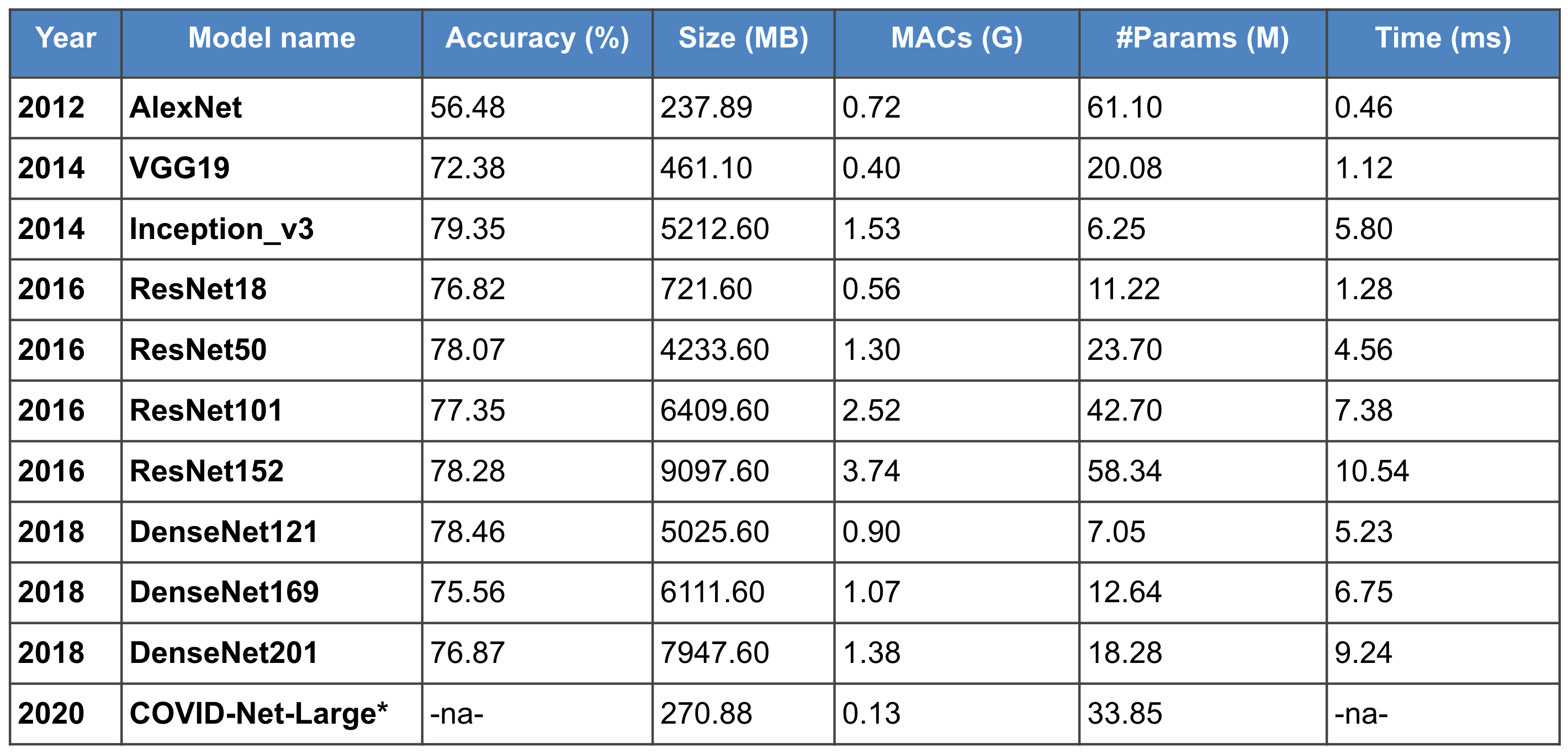
The table below was compiled by Deeplite to illustrate the problem. in the evolution of DNN architectures over the past decade and their consistent growth in depth and size. Here, you can very well see how the improvement in the model accuracy correlates to the increase in memory size (MB), the computational cost (Giga MACs), number of parameters (Million), and the inference time (for batch size 128).

The primary reason for the explosion in this complexity is the necessity for a DNN model’s success, measured by its correctness, accuracy, error rate, F1 score, and an area under the curve (AUC). For instance, in autonomous cars, a ML failure can be hazardous or even life-threatening. Therefore, a deeper DNN architecture could provide competitive results on benchmark datasets across all applications, while consuming these extensive state-of-art DNN models in multiple production-ready real-time systems is a challenge due to in-device memory constraints and inference time bottlenecks.
For instance, let’s break down how costly a single convolution layer can be... (typically, the learnable parameters of a DNN model include weights and biases. But let’s do just a brief exercise and observe only the weight parameters for now).
Imagine a convolution layer with 512 kernels, each having (3 x 3) weight values. This layer’s input shape (128 x 224 x 224 x 256) yields the output shape of (128 x 224 x 224 x 512), assuming padding and stride of 1. Such a convolution layer will have (3 x 3 x 256 x 512) several weight values to learn. Each weight value is represented as a float32 data type, occupying 4bytes of memory (32 bits). Thus, the memory required to store these weight parameters is (3 x 3 x 256 x 512 x 4) bytes = 4.5MB.
In addition, this layer produces an output of shape (128 x 224 x 224 x 512) and the memory required to store this output from the layer is (128 x 224 x 224 x 512 x 4) bytes = 12.25GB. During training and backpropagation, this layer would need to compute a gradient of shape (128 x 224 x 224 x 512), requiring an additional memory of (128 x 224 x 224 x 512 x 4) bytes = 12.25GB. Thus, due to the addition of one standard convolution layer, the additional memory required is:
As seen in the example above, successful DNN architectures can become very large and computationally costly. The memory, time, hardware, and energy constraints prevent deep learning from penetrating and enhancing multiple industry applications. There is an immediate need for optimizing and compressing these DNN architectures to be able to consume them. At Deeplite, we embrace the importance of DNN model optimization to enable AI applications even on very constrained resources and making it useful for our everyday lives. Thus, we decided to share our knowledge in this multi-part DNN optimization blog series and demonstrate how we tackle the challenges of producing an easy-to-use DNN model optimization framework.
Optimization is a pretty vast notion and can imply many things. So, let’s look at what DNN architecture optimization actually entails.

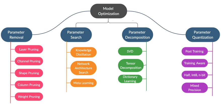
Fundamentally, DNN architecture optimization is about reducing the number of parameters in your model. Fewer parameters require less memory space, which results in a smaller number of computations and improves the inference time. There are multiple methods explored in the literature that reduce the number of parameters. These techniques, as shown in the following figure, can be broadly grouped into four categories: 1) parameter removal, 2) parameter search, 3) parameter decomposition, and 4) parameter quantization.
Note, this categorization highlights the key techniques for optimization and is not exhaustive.

Let’s talk more about each of these DNN optimization techniques, how do they differ from each other, their pros and cons, and if is there one that would fit your case better.
Have you ever heard of the phrase ‘DNN model is overparameterized with redundant weights’? This basically means that if a DNN model has a gazillion weight parameters, not all of them will contribute to obtaining the desired output. Thus, they are useless and can be eliminated from the model.
The parameter removal technique’s primary aim is to identify those ‘useless’ weights that do not contribute to the output and eliminate them to achieve a smaller model. This can be accomplished by either pruning the weights or distilling the entire model. This technique holds challenges such as:
DNN model optimization can also be viewed as a search task. Let's say we have a set of all possible different DNN models, and we search for the model with fewer parameters than the original model yet providing similar accuracy performance. In this case, the original model is called the teacher, and the new one we are searching for is called the student.
The student model learns from the weights of the teacher. Then, we either distill the student model from the teacher model or search the student model architecture from scratch. For example, Lottery Ticket Hypothesis is a popular new technique for model optimization as a search problem!
Depending on the number of hyperparameters in consideration, the search space can become ridiculously large. So the downfall of this technique is, searching and finding a suitable student model can be time-consuming and resource-intensive. Additionally, the sampled new student model’s accuracy is unknown until sufficient fine-tuning is performed on the teacher’s training data. This additional overhead of more training and fine-tuning steps adds to the challenge of time and resource requirements. In practice, unconstrained, real-time systems searching for the appropriate student model might not be efficient.
Here is how decomposition works. We fragment a vast weight matrix (or tensor) into smaller pieces, such that there is minimal information losses minimal information loss as possible.
Imagine a fully connected neural network with hidden layers of (100, 200) neurons each. The weight matrix connecting these two layers would have the shape of 100x200=20000 weight parameters. But what if we decompose each layer in this network into a set of smaller layers with (100, 2, 2, 200) neurons each? In this case, the weight matrix connecting these sets of layers would be of the shape (100 x 2) + (2 x 2) + (2 x 200) = 604 weight parameters, resulting in ~97% compression.
The weight decomposition technique’s drawback is the difficulty of finding the right decomposition rank for a given tensor of weight, allowing us to retain as much information as possible while still computing smaller matrix values.
For the sake of the experiment, let’s assume that our DNN model is not overparameterized, and every single weight value in it is important. Given that, each weight value will require 4bytes of memory with a precision of float32. The idea behind quantization is to reduce the memory needed for each weight value. Converting the precision of all the weight values to Int16 reduces the model’s size to 50%. Logically altering the precision of weight values to Int8, 4bits, 2bits, or even binary (1 bit) will further reduce the model size.
Instead of quantization, we can also perform weight values’ binning, keeping the original precision of weight values. Let’s assume that a convolution layer has a weight tensor of shape (3 x 3 x 256 x 512) and could contain all 1179648 unique and different float32 values. The idea behind binning is to reduce the number of possible unique values in the weight tensor. Hence, instead of 1179648 unique values, we can reduce the number of unique values to 4, requiring only 2bits to store all the required weight values.
The primary downside of the quantization and binning technique is that it usually results in much information loss. The more aggressive the quantization is, the less hope we have for retaining the right information. For example, a 2bit quantization can store only four unique weight values.
While every optimization technique has its advantages, challenges, and drawbacks, Deeplite decided to provide you with a summary of pitfalls you might want to watch out for when conducting your optimization in a production setup.
How do we reduce the number of parameters, but retain an equivalent accuracy performance? Retaining the performance includes more than one possible loss function, including customized ways to evaluate networks. An optimized model is only useful if functional accuracy is preserved on the relevant criteria (cross-entropy, SME, mean average precision (mAP), F1 score, IoU etc.)
There are multiple metrics to optimize: the number of parameters, model size, inference time, the computational cost in terms of MACs etc. Optimizing even one of those metrics is challenging, so watch out when you are trying to optimize them together.
Different applications might require one or a few of these metrics to be highly optimized while overlooking or even ignoring others.
For example, real-time systems would require the inference time to be low but would not expect a much smaller model size. Make sure to guide your model optimization to favor these specific metrics depending on your DNN model’s purpose.
The generic implementation of Conv2D operation in popular libraries such as PyTorch, Tensorflow, Keras, or Caffe2 does not support specific pruning and quantization methods.
How do we implement custom convolution operation with similar efficiency? Different implementations of convolution operations exist between frameworks and custom operations are not always supported or easy to optimize using hand-crafted techniques, particularly across multiple networks. One of the difficulties for optimization is to support and implement various operations while improving the model performance.
The compiler and the hardware execution of the optimized model can be challenging. Most optimization techniques are targeted for GPU or server-class CPU execution. Can we optimize DNN architectures for different and specialized hardware such as Android, Arduino, and various ASICs now entering the fray? Furthermore, how might we learn optimal network architectures that provide insight into potential hardware optimizations that maximize performance?
Considering the complexity of optimizing DNN models and the opportunity presented when DNNs are optimized successfully, there is a significant need for a black-box optimization framework, where the end-user could just provide the trained model, the training dataset, and an easy way to provide constraints for optimization. End-user experience and usability is a crucial requirement in consuming optimization in production pipelines.
One could argue that there are plenty of research papers and blogs, and technical articles that aim to address and solve many of the above challenges. However, apart from the above technical challenges, some non-technical difficulties prevent DNN optimizations from penetrating into widespread applications:

![]() To maximize the opportunity created by optimized DNN models, engineers in multiple markets and application domains as well as researchers are now able to automatically optimize their models using Deeplite’s optimization software. Deeplite implements a complete black-box, very easy-to-use and integrated framework for DNN model optimization. All you need to do is provide the pretrained model with the training and test data using the on-premise pip package or dockerized engine.
To maximize the opportunity created by optimized DNN models, engineers in multiple markets and application domains as well as researchers are now able to automatically optimize their models using Deeplite’s optimization software. Deeplite implements a complete black-box, very easy-to-use and integrated framework for DNN model optimization. All you need to do is provide the pretrained model with the training and test data using the on-premise pip package or dockerized engine.
Then you provide any constraints or guidelines for optimizing the model, such as the maximum tolerance in accuracy reduction or error-rate permissible in your case and desired compression level Deeplite uses a patented optimization engine called Neutrino™ to understand the model's complexity and perform the most suitable optimization, with minimal effort required from the end-user.
You can also choose between different optimization levels, such as Level 1, Level 2, and Level 3. Each deeper level provides more aggressive optimization at the cost of additional time in obtaining the optimized model.
Here is how it looks in action.
As seen in the demo, by using Deeplite you won't have to struggle with implementing complex pruning techniques or custom operations on top of the DNN architectures. All the heavy lifting is removed by Deeplite’s easy-to-use optimization engine.
Deeplite's Neutrino™ engine is available on-premise, via a Python pip distribution. It is programmable and highly integrable in existing workflows and development lifecycles. Deeplite also aims at providing a library agnostic interface for providing model optimization, supporting PyTorch and Tensorflow models.
Our engine uses a combination of different weight reduction techniques along with a sophisticated search, to find the most optimized model with as minimal searching cost as possible.
That's it for now! We hope you enjoyed reading our article! We certainly will be publishing more posts around challenges in DNN model optimization. Sign up for our blog newsletter if you want to stay tuned.
Let us know if you have any questions or would like us to cover any other topics in this blog by leaving a comment below.

Anush Sankaran
Senior Research Scientist at Deeplite
Medium.com: @anush.sankaran
Twitter: @goodboyanush

Anastasia Hamel
Digital Marketing Manager at Deeplite
Medium.com: @anastasia.hamel
Twitter: @anastasia_hamel