DNN Model Optimization Series: Part III - Achieve up to 30x DNN Model Compression (while maintaining accuracy!)

Welcome back to the DNN model optimization series! Our recent paper on Deeplite’s unique optimization software, Neutrino™, won the “Best Deployed System” award at Innovative Applications of Artificial Intelligence 2021. For this occasion, we decided to dedicate this issue of the DNN model optimization series to a deep-dive into the champion research paper.

AI and deep learning, particularly for edge devices, have been gaining momentum and promising to empower the digitalization of many vertical markets. Despite all the excitement, deploying deep learning is easier said than done! We already looked at why you need to optimize your DNN models in one of our previous blog posts. Let’s look at ‘how’ Deeplite’s Neutrino™ framework addresses the ever-larger AI models’ optimization and paves the way for easy deployments into increasingly constrained edge devices.

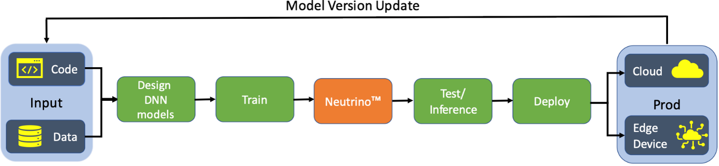
Neutrino™ is an end-to-end black-box platform for fully automated DNN model compression that maintains the model accuracy. It can be seamlessly and smoothly integrated into any development and deployment pipeline, as shown in the figure below. Guided by the end-user constraints and requirements, Neutrino™ produces the optimized model that can be further used for inference, either directly deployed on the edge device or in a cloud environment.

Deeplite’s Unique Way to Compress DNN Models

What will you need to get started?

1. Your pre-trained DNN model, M,
2. The actual train-test data split you used to train the model, DL_train and DL_test, and
3. The following set of requirements to guide the optimization:

• Delta: The acceptable tolerance of accuracy drop with respect to the original model, for example, 1%.
• Stage: The two different compression stages, while stage 1 is less intensive compression requiring fewer computational resources, stage 2 provides more aggressive compression using more resources and time.
• Device: Perform the entire optimization and model inference in either CPU, GPU, or multi-GPU (distributed GPU environment).
• Modularity: The end-user can customize multiple parts of the optimization process for Neutrino™ to adapt to more complex scenarios. This customization includes specialized data-loaders, custom backpropagation optimizers, and intricate loss functions that their native library implementation allows.

The algorithm that we used to understand, analyze, and compress the DNN model automatically for a given dataset is explained below.

The Four Components of Neutrino™

1. Neutrino™ Model Zoo: To ease the use for the end-user, a collection of popular DNN architectures with trained weights on different benchmark datasets are provided as Neutrino™ Zoo.
2. Conductor: The purpose of the conductor is to collect all the provided inputs, understand the given requirements, and orchestrate the entire optimization pipeline, accordingly.
3. Exploration: It’s a high-level coarse compression stage, where the composer selects different transformation functions for the different layers in the DNN model.
4. Annealing: It’s a fine-grained aggressive compression stage to obtain the maximum possible compression in the required tolerance of accuracy.

The Process

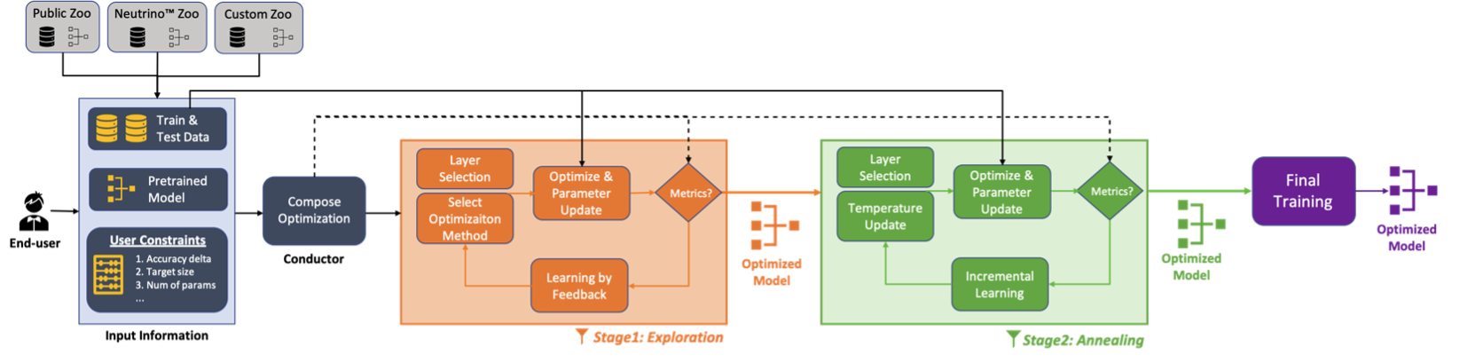
In one of our blog posts, we already answered the top 10 questions about the model compression process. To briefly explain, at Deeplite, we dynamically combine different optimization methods for different layers in a model to create a beautiful result, achieving maximum compression with minimal accuracy loss (and when we say minimal, we mean it! Look at the outcomes below).

Let’s look at an example here. Our pre-trained model has N optimizable layers: {L1, L2, ..., LN}. In a typical CNN model, the convolutional layers and the fully connected layers are optimizable, while the rest of the layers are ignored from the optimization process. The conductor analyzes the training data size, the number of output classes, model architecture, and optimization criteria, delta, and produces a composed list, CL = {c1, c2, ..., cN} of different transformation functions for different layers in the model. For any layer, L_i, in the model, the composed function ci looks like this:

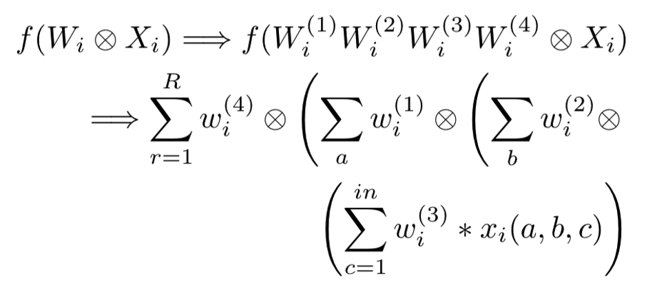
The challenge is to find an ideal size r that produces good compression retaining the model’s robustness. When r is equal to the actual size of the weight tensor of the layer, r = size(Wi), there is an over-approximation of the transformation with very low compression. However, a very small size, r → 0, produces a high compression with a lossy re-construction of the transformation.

Stage 2 optimization aims to perform aggressive compression and obtain the maximum possible compression in the required accuracy tolerance. For example, if the delta of accuracy is 1%, and stage 1 produces a 4x compression with an accuracy drop of 0.6%, stage 2 aims to advance the compression with the delta going as close as possible to 1%.

How Do We Measure the Optimization and Compression Performance?

Here are the metrics we use to measure the amount of optimization and performance of Neutrino™.

Accuracy: We measure the top-1 accuracy (%) of the model. Successful optimization retains the accuracy of the original model.

Model Size: We measure the disk size (MB) occupied by the trainable parameters of the model. Smaller model size enables models to be deployed into devices with memory constraints.

MACs: We measure the model’s computational complexity by the number (billions) of Multiply-Accumulate Operation (MAC) computed across the layers of the model. The lower the number of MACs, the better optimized the model is.

Number of Parameters: We measure the total number (millions) of trainable parameters (weights and biases) in the model. Optimization aims to reduce the number of parameters.

Memory Footprint: We measure the total memory (MB) required to perform the inference on a batch of data, including the memory required by the trainable parameters and the layer activations. A lower memory footprint is achieved by better optimization.

Execution Time: We measure the time (ms) required to perform a forward pass on a batch of data. Optimized models have a lower execution time.

DNN Model Compression Results Using Neutrino™

All the optimization experiments are run with an end-user requirement of accuracy delta of 1%. The experiments are executed with a mini-batch size of 1024, while the metrics are normalized for a mini-batch size of 1. All the experiments are run on four parallel GPU, using Horovod, and each GPU is a Tesla V100 SXM2 with 32GB memory.

Depending on the architecture of the original model, it can be observed that the model size could be compressed anywhere between ∼3x to ∼30x. VGG19 is known to be one of the highly over-parameterized CNN models. As expected, it achieved a 29.22x reduction in the number of parameters with almost ∼12x compression in the overall memory footprint and ∼an 8.3x reduction in computation complexity. The resulting VGG19 model occupies only 2.6MB as compared to the original model requiring 76.6MB.

The performance of Neutrino™ on large-scale vision datasets produces around ∼23.5x compression of ResNet18 on Imagenet16 and VWW datasets. The optimized model requires only 1.8MB as compared to the 42.6MB needed for the original model.

Stage 1 vs. Stage 2 Compression

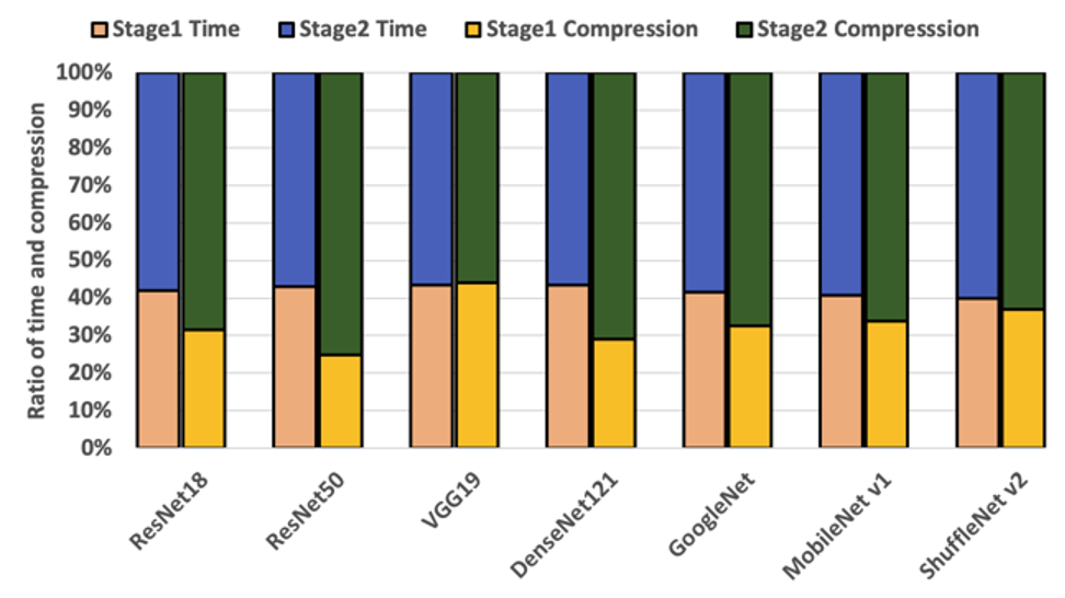
Crucially, it can be observed that Stage 2 compresses the model at least 2x more than Stage 1 compression. The overall time taken for optimization by Neutrino™, including Stage 1 and Stage 2, is shown in the figure below. It can be observed that most of the models could be optimized in less than ∼2 hours. Complex architectures with longer training times, such as Resnet50 and DenseNet121, take around ∼6 hours and ∼13 hours for optimization.

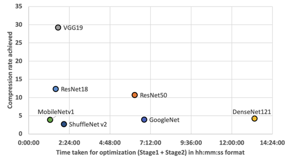
The comparison between the time taken for Stage 1 and Stage 2 compression is visually shown in the below figure. It can be observed that almost 60−70% of the overall optimization is achieved in Stage 2, while Stage 1 consumes less than ∼40% of the overall time required. This differentiation acts as a key feature of Neutrino™, where end-users who need quick optimization with less resource consumption can choose Stage 1. In contrast, those needing aggressive optimization can choose Stage 2 optimization.

Production Results of Neutrino™

Deeplite’s Neutrino™ is deployed in various production environments, and the results of the various use-cases obtained are summarized in the table below. To showcase the efficiency of Neutrino™’s performance, the optimization results are compared with other popular frameworks in the market, such as (i) Microsoft’s Neural Network Interface (NNI), Intel’s Neural Network Distiller, and (iii) Tensorflow Lite Micro. It can be observed that Neutrino™ consistently outperforms the competitors by achieving higher compression with better accuracy.

How to Use Neutrino™?

The Neutrino™ framework is completely automated and can optimize any convolutional neural network (CNN) based architecture with no human intervention. Neutrino™ framework is distributed as Python PyPI library or Docker container, with production support for PyTorch and early developmental support for TensorFlow/Keras.

That’s it for now, folks! Remember, compression is a critical first step in making deep learning more accessible for engineers and end-users on edge devices. Unlocking highly compact, highly accurate intelligence on devices we use every day, from phones to cars and coffee makers, will have an unprecedented impact on how we use and shape new technologies.

Do you have a question or want us to look into other AI model optimization topics? Leave a comment below. We’ll be happy to follow up!

Interested in signing up for a demo of Neutrino™? Please refer to this link.

Meet the blog authors:

Anush Sankaran
Senior Research Scientist at Deeplite
Medium.com: @anush.sankaran
Twitter: @goodboyanush

Anastasia Hamel
Digital Marketing Manager at Deeplite
Medium.com: @anastasia.hamel
Twitter: @anastasia_hamel